print(__doc__)import matplotlib.pyplot as pltimport numpy as npimport seaborn as snssns.set_context("poster")rng = np.random.RandomState(18)f, ax = plt.subplots(figsize=(8, 8))# generate some data pointsy = np.array([3.65284, 3.52623, 3.51468, 3.22199, 3.21])z = np.array([0.43, 0.45, 0.6, 0.4, 0.211])y_2 = np.array([3.3, 3.6])z_2 = np.array([0.58, 0.34])# plot the majority and minority samplesax.scatter(z, y, label="Minority class", s=100)ax.scatter(z_2, y_2, label="Majority class", s=100)idx = rng.randint(len(y), size=2)annotation = [r"$x_i$", r"$x_{zi}$"]for a, i inzip(annotation, idx): ax.annotate(a, (z[i], y[i]), xytext=tuple([z[i] +0.01, y[i] +0.005]), fontsize=15)# draw the circle in which the new sample will generatedradius = np.sqrt((z[idx[0]] - z[idx[1]]) **2+ (y[idx[0]] - y[idx[1]]) **2)circle = plt.Circle((z[idx[0]], y[idx[0]]), radius=radius, alpha=0.2)ax.add_artist(circle)# plot the line on which the sample will be generatedax.plot(z[idx], y[idx], "--", alpha=0.5)# create and plot the new samplestep = rng.uniform()y_gen = y[idx[0]] + step * (y[idx[1]] - y[idx[0]])z_gen = z[idx[0]] + step * (z[idx[1]] - z[idx[0]])ax.scatter(z_gen, y_gen, s=100)ax.annotate(r"$x_{new}$", (z_gen, y_gen), xytext=tuple([z_gen +0.01, y_gen +0.005]), fontsize=15,)# make the plot nicer with legend and labelsns.despine(ax=ax, offset=10)ax.set_xlim([0.2, 0.7])ax.set_ylim([3.2, 3.7])plt.xlabel(r"$X_1$")plt.ylabel(r"$X_2$")plt.legend()plt.tight_layout()plt.show()
Automatically created module for IPython interactive environment
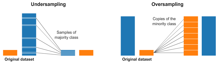
under-sampling
Illustration of the definition of a Tomek link
print(__doc__)import matplotlib.pyplot as pltimport seaborn as snssns.set_context("poster")
Automatically created module for IPython interactive environment